The focus of this article will be on how you can analyze scraped data with two of the most powerful and widely used Python libraries: Pandas and Matplotlib.
Let’s get into it!
Before proceeding, let me thank Decodo, the platinum partner of the month, and their Scraping API.
Scraping made simple - try Decodo’s All-In-One Scraping API free for 7 days.
Pandas is an open-source library built on Python for data analysis and data manipulation. It provides data structures designed specifically to handle tabular datasets called dataframes:
A Pandas dataframe
A pandas dataframe is a two-dimensional table where each column represents a variable, and each row stores a set of corresponding values. The data stored in a dataframe can be numeric, categorical, or textual. This allows Pandas to manipulate and process diverse datasets.
Below are Pandas’ main features:
Data import and export: You can import and export data in different formats such as CSV, SQL, Parquet, and spreadsheets.
SQL-like functionalities: You can manipulate dataframes with functionalities that are similar to SQL. This involves merging dataframes, filtering data, grouping data, and more.
Simplicity of use and thorough documentation: Pandas is the top-notch choice for preparing data for analytics and machine learning if you use Python. So it has a very curated documentation. It is also easy to use, even if you are a beginner.
Smooth integration: As it is built on top of Python, it seamlessly integrates with every other Python library.
This episode is brought to you by our Gold Partners. Be sure to have a look at the Club Deals page to discover their generous offers available for the TWSC readers.
Matplotlib is a popular data visualization library. You can use it to create a diverse set of common plots like line charts, bar charts, histograms, and more. It provides you with a wide array of personalization possibilities that range from adding legends to charts, changing colors, adding charts’ titles, and more.
The following is a list of its main features:
Data type integration: Matplotlib is built to work with NumPy arrays and Pandas dataframes. So, basically, you can create your Pandas dataframe, filter and clean the data, and create plots smoothly.
Python compatibility: It is written in Python, so it is compatible with any other Pythonic library you use.
Full personalization and customization: With Matplotlib, you can customize the colors of your plots, the font you use and its dimensions, and many more parameters with just a few lines of code.
Wide array of plots: It allows you to plot a wide array of plots, from scatterplots to histograms.
Before continuing with the article, I wanted to let you know that I've started my community in Circle. It’s a place where we can share our experiences and knowledge, and it’s included in your subscription. Enter the TWSC community at this link.
Analyzing Scraped Data With Pandas And Matplotlib: Step-by-step Tutorial
In this step-by-step tutorial section, you will learn how to use Pandas and Matplotlib to analyze scraped data. First, note that, in order to use Pandas, you need tabular data. So, you have two possibilities:
You scrape data that is already in a tabular format.
You scrape unordered data and manipulate it to make it tabular.
For this tutorial, the target page reports the Gross Domestic Product (GDP) per year in the United States, and is the following:
Perfect! Your system matches all the requirements needed for proceeding with the tutorial.
Prerequisites
Before proceeding with the tutorial, you have to set up a Jupyter Notebook. From the main folder (data_analysis/), type the following via the CLI to launch a new Jupyter Notebook:
jupyter notebook
This command will open a new browser instance. Click on New > Python3 (ipykernel) to create a new Jupyter Notebook file:
Creating a new Jupyter Notebook file
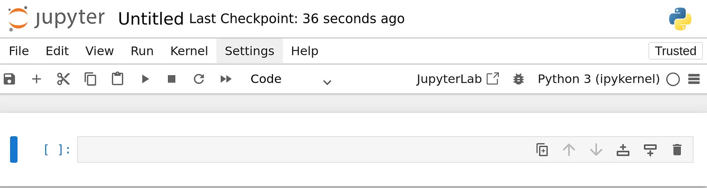
This is what it looks like:
A new Jupyter Notebook file
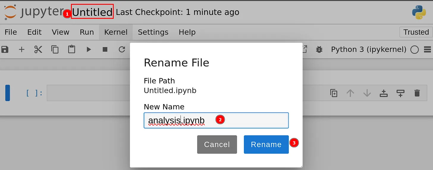
Click on Untitled and rename the file, for example, as analysis.ipynb:
Renaming a Jupyter Notebook file
Very well! Everything is ready for proceeding with the actual tutorial.
If you analyze the target page with the Chrome Developer Tools, you can see that the CSS selector that defines the table is .table:
The table’s CSS selector
Also, each row is contained inside a <tr>:
The rows’ CSS selectors
So, to retrieve all the data and save it into a CSV file, you can write the following code in scraper.py:
import requests
from bs4 import BeautifulSoup
import csv

# URL of the website
url = “<https://www.worldometers.info/gdp/us-gdp/>”

# Send a GET request to the website
response = requests.get(url)
response.raise_for_status()

# Parse the HTML content
soup = BeautifulSoup(response.text, “html.parser”)

# Locate the table
table = soup.find(”table”)

# Extract table headers
headers = [header.text.strip() for header in table.find_all(”th”)]

# Extract table rows
rows = []
for row in table.find_all(”tr”)[1:]:  # Skip the header row
    cells = row.find_all(”td”)
    row_data = [cell.text.strip() for cell in cells]
    rows.append(row_data)

# Save the data to a CSV file
csv_file = “us_gdp.csv”
with open(csv_file, mode=”w”, newline=”“, encoding=”utf-8”) as file:
    writer = csv.writer(file)
    writer.writerow(headers)  # Write headers
    writer.writerows(rows)    # Write rows

print(f”Data has been saved to {csv_file}”)
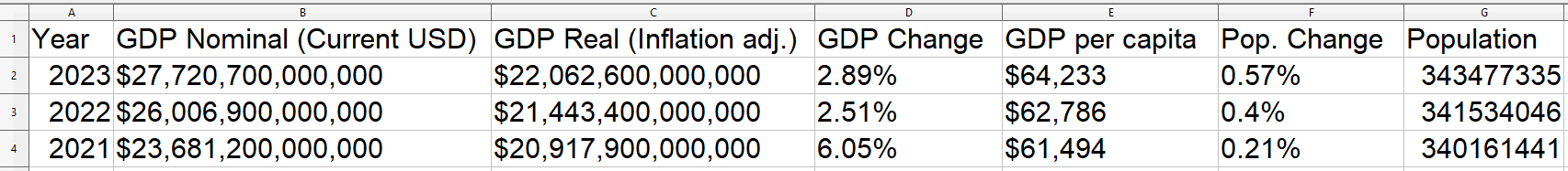
At the end of the process, you can open the us_gdp.csv file to verify that it has been successful:
The resulting CSV file
Hooray! You scraped the target data. Now you are ready to start manipulating it with Pandas.
Step #2: Open The CSV With Pandas
In the first cell of your analysis.ipynb Notebook, import Pandas and Matplotlib as follows:
import pandas as pd
import matplotlib.pyplot as plt
This is a standard and worldwide-recognized notation. It is used to make the code shorter, without writing the entire libraries’ names.
Run the cell to make the import effective by typing SHIFT + ENTER.
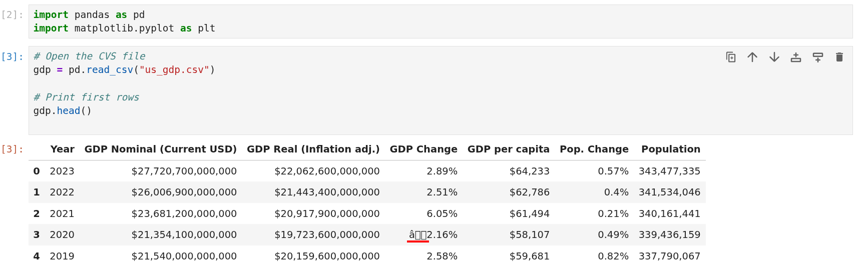
In the second cell, import the CSV file containing the scraped data and visualize the first 5 rows:
# Open the CVS file
gdp = pd.read_csv(”us_gdp.csv”)

# Print first rows
gdp.head()
In this code:
The read_csv() method opens the CSV file and, under the hood, transforms it into a Pandas dataframe.
The head() method returns the first 5 rows of the dataframe.
The image below shows the current situation in your Notebook:
The first cells of the Jupyter Notebook
As the image shows, the dataframe has the following issues that must be fixed:
The GDP Change column has some non-recognized characters.
All the columns, apart from Year, have the % or $. This means that the data inside is not numbers.
One way to verify that the values in the columns, apart from Year, are not numeric is by using the describe() method, which reports a statistical summary of the dataframe. By typing gdp.describe() you will obtain the following:
Initial statistics of the dataframe
As the image shows, the statistics are reported only for the Year column because it is the only column that stores numerical values.
Very well! You opened your first CSV with Pandas as a dataframe. You are now ready to manipulate the data.
First of all, this dataset has two rows with non-recognized characters. The issue may be due to how the data is actually stored in the table in the target page. In such cases, you have basically two options:
You remove the rows.
You manually change the values in the CSV and load the CSV again in the Jupyter Notebook (re-run the cell after you manually changed the values in the CSV).
Since the data is a few, I decided to change the values in the columns manually—And yes, Something like that is always part of the data manipulation process! Note that the unrecognized character is a minus sign (”-”). So, if you were to delete those rows, you would lose all the negative numbers stored in the CSV. This is a kind of consideration to account for when cleaning data.
Now, you have to transform the values in the columns to be numbers. But before doing that, you have to remove the $ and % signs. You can do so with the following code:
# Remove the $ and %
gdp = gdp.apply(
    lambda s: (s.astype(str)
                 .str.replace(r’[\\$,%]’, ‘’, regex=True)
                 .str.replace(’,’, ‘’, regex=False)
                 .str.strip())
)

# Transform values to numbers
gdp = gdp.apply(pd.to_numeric, errors=’coerce’)
The above code uses:
The replace() method, along with regex, to remove the dollar and percentage symbols.
The to_numeric() method to transform the values into numbers.
Now, if you type gdp.describe(), you will obtain the statistical summary for each column, confirming that the values are all numbers:
The dataframe’s data without symbols
As a final manipulation step, you may want to rename the columns to make them more descriptive. For example, you can specify the unit of measure where this applies—for instance, USD or %, as it applies in this case. To do so, use the following code:
# rename columns
gdp = gdp.rename(columns={”GDP Nominal (Current USD)”:”GDP Nominal [$]”,
“GDP Real (Inflation adj.)”:”GDP Inflation Adjusted [$]”,
“GDP Change”:”GDP Change [%]”,
“GDP per capita”:”GDP per capita [$]”,
“Pop. Change”:”Pop. Change[%]”}
)
Below is the result:
Renaming columns in Jupyter Notebooks
So, use the rename() method to rename columns and make them more descriptive, if you need it.
Wonderful! You completed your first data cleaning and manipulation task. You are now ready to visualize the data.
Step #4: Data Visualization
Suppose you want to visualize the trend of the nominal GDP over the years. To do so, write the following code in a new cell:
# Select columns and sort values by year
gdp_plot = (gdp[[”Year”, “GDP Nominal [$]”]]
           .sort_values(”Year”))

# Plot in trillions for readable axis
gdp_trillions = gdp_plot[”GDP Nominal [$]”] / 1e12

fig, ax = plt.subplots(figsize=(9,5))
ax.plot(gdp_plot[”Year”], gdp_trillions, marker=”o”, linewidth=2, color=”#2a7ae2”)

# Set title and labels
ax.set_title(”GDP Nominal by year in the US”)
ax.set_xlabel(”Year”)
ax.set_ylabel(”Nominal GDP in the US [trillions of $]”)
ax.grid(True, alpha=0.3)

ax.set_xticks(gdp_plot[”Year”])
plt.xticks(rotation=90) # Rotate 90° x values for readability

# Show layout and plot
plt.tight_layout()
plt.show()
This code does the following:
Selects only the columns needed for the plot (”Year” and “GDP Nominal [$]”) and sorts the values per year.
Divides the values of the “GDP Nominal [$]” by trillions for better readability.
Plots the values per year, defining the type of marker, the color, and the width of the line connecting the dots.
Sets the labels with set_title, set_xlabel, etc*.*
Rotates the values on the x-axis (the years) by 90° with plt.xticks(rotation=90) for better readability.
Shows the layout and plots the graph.
The result is in the following image:
A line plot with Matplotlib of the nominal GDP per year in the US
As a final plot, you may be interested in a bar chart that shows how the percentage of the GDP has changed over the years. To do so, type the following code into a new cell of your Notebook:
# Prepare data
df = gdp[[”Year”, “GDP Change [%]”]].sort_values(”Year”).copy()
x = df[”Year”]
y = df[”GDP Change [%]”]

# If stored as fractions (0–1), convert to percent
if y.max() <= 1:
    y = y * 100

# Set color negatives red and positives green
colors = [”#2ca02c” if v >= 0 else “#d62728” for v in y]

# Plot bar chart
fig, ax = plt.subplots(figsize=(9, 5))
bars = ax.bar(x, y, color=colors, edgecolor=”black”, linewidth=0.5)

# Define labels
ax.set_title(”GDP Change by Year”)
ax.set_xlabel(”Year”)
ax.set_ylabel(”GDP Change [%]”)
ax.set_xticks(x)
plt.xticks(rotation=90) # Rotate 90° x values for readability
ax.grid(axis=”y”, alpha=0.3)

# Plot layout and show chart
plt.tight_layout()
plt.show()
Here is what this code does:
Selects the columns you are interested in and stores their values as x and y.
Manages the colors of the plotted values. In particular, the bars will be colored in red if the value is negative. If positive, the color will be green.
Defines the labels of the axis and the title of the chart.
Below is the resulting plot:
A bar plot in Matplotlib of the GDP percentage change per year in the US
As discussed in step #3, if you had removed the rows with unrecognized characters without further investigations, you would have lost the negative values. With this plot, you can visually quantify the mistake you would have made.
Et voilà! You have created two plots with Matplotlib from a Pandas dataframe obtained by scraping the data.
The Web Scraping Club is a reader-supported publication. To receive new posts and support my work, consider becoming a free or paid subscriber.
Conclusion
In this article, you have learned how to start analyzing scraped data with Pandas and Matplotlib. These two libraries stand at the core of modern data analytics with Python, so they are a must-know. You can find the code used in the GitHub repository at this link.
Still, you have also learned how easy it is to use them to manipulate data and, especially, to create customized plots.
So, let us know in the comments: are you analyzing the data you scrape? What’s your experience with those libraries?