Over the last decade, we have seen the same mantra repeated almost daily: “data is the new oil.” But like crude oil, raw data isn't valuable on its own. That's where the magic of predictive analytics comes in: turning vast amounts of information into actionable forecasts. But what if you don't have access to large, proprietary datasets? Well, in this case, you basically have only one choice: web scraping.
Web scraping is a powerful technique for data acquisition, and I've always been fascinated by what you can do with that data once it's acquired. One of the most exciting applications is using it to predict future outcomes.
In this article, you'll explore the intersection of these two fields: web scraping and predictive analytics. I'll break down what predictive analytics means and discuss why web scraping is an important asset to it. Then, you'll go through a complete step-by-step tutorial to learn how to scrape data and then make predictions with it using predictive modeling.
Ready? Let’s dive into it!
Before proceeding, let me thank NetNut, the platinum partner of the month. They have prepared a juicy offer for you: up to 1 TB of web unblocker for free.
Predictive analytics is the practice of using historical data to predict future events. At its core, it’s all about identifying the likelihood of future outcomes based on patterns found in the past. So, you can think of predictive analytics as a form of technological fortune-telling, but one that's grounded in data and statistics rather than a crystal ball.
Let me tell you this more clearly: predictive analytics is nothing more than applied mathematics. I hope I don't disappoint you, but someone had to say this harsh truth! I know that there is a lot of hype out there about “predicting the future”, but there’s no involvement of black magic here. The tutorial at the end of this article will clearly show you this: you’ll apply a mathematical model that learns the patterns inside the data. Once the model has its knowledge on a training dataset, it is used to predict the output value(s) of data it has never seen on a test dataset.
It makes more sense now, right? I feel you! However, the processes are not that easy, as you can imagine. So, let’s focus on an example to help you gain an understanding of the processes under the hood.
In the world of Machine Learning (ML) and Deep Learning (DL), predictive models can analyze complex, multi-dimensional data to find subtle relationships that a human analyst would almost certainly miss. For example, a predictive model might forecast sales based on last year's numbers. A more advanced ML model could predict the same sales by analyzing not just historical sales, but also competitor pricing, customer reviews, social media sentiment, and even macroeconomic indicators.
This is where terms like "training a model" come from. You "train" an algorithm by feeding it massive amounts of historical data, complete with the outcomes that actually occurred, in the case of supervised learning. The model learns the patterns associated with those outcomes. Once trained, you can give it new, current data, and it will produce a prediction—a calculated guess—about what will happen next.
But before proceeding, you read above about ML and DL as predictive models. But how do they differ? Well, to simplify things, the jargon says that you can refer to machine learning even in the case of deep learning. This is because DL is a subset of ML:
This episode is brought to you by our Gold Partners. Be sure to have a look at the Club Deals page to discover their generous offers available for the TWSC readers.
Why is Web Scraping Useful for Predictive Analytics?
The single most important ingredient for any predictive analytics project is data. Lots of it. The more relevant and high-quality data you can feed your model, the more accurate its predictions will be.
But here is the point: while many large companies have the advantage of massive internal datasets collected over the years, most businesses and individuals don't have that luxury. This is where web scraping comes into play. The internet is the largest, most dynamic database in human history, and web scraping is the key to unlocking it. It allows you to systematically collect public data from websites, providing the raw material for your predictive models.
Think about the possibilities:
An e-commerce business could scrape competitor websites to gather data on pricing, promotions, and product availability. By feeding this data into a model, they could predict how a competitor's price drop will affect their own sales and adjust their strategy proactively.
A hedge fund could scrape financial news sites and social media to gauge market sentiment, helping it predict stock price movements.
The applications are virtually endless and span across industries, from real estate to marketing and beyond. However, the basics of why web scraping is important for predictive analytics remain. To put it concretely, here are some of the key reasons why web scraping is a superpower for any machine learning project:
Massive data acquisition: Machine learning algorithms—particularly in the deep learning domain—are notoriously data-hungry. Their performance is directly tied to the quantity of training data you can provide. Web scraping is the primary method for acquiring the massive datasets needed for robust model training, accessing information that isn't available in neatly packaged APIs or internal databases.
Broadening data horizons: Even if you have a solid internal dataset, it likely represents only one part of the picture. By scraping various sources, you can supplement your primary datasets, introducing new features and perspectives that can dramatically improve your model's understanding of the world. This also prevents the biases that come from a single source of information.
Access to real-time insights: The world changes fast, and static datasets quickly become old. Web scraping is the solution for keeping your data current. So, web scraping is essential for any application where predictions depend on timely information, such as sentiment analysis of breaking news, dynamic pricing strategies, or financial market analysis.
Boosting accuracy and robustness: Often, the bottleneck to a better model isn't a fancier algorithm—it's more data. Scraping the web is a direct way to acquire additional data for training, which can significantly boost your model's predictive accuracy. It also provides new, unseen data perfect for validating your model's performance against real-world scenarios.
Gauging the market's temperature: To predict market trends, you first need to understand them. Scraping product reviews, social media discussions, and news articles allows you to quantify public sentiment and identify emerging trends. This "voice of the consumer" data can be an invaluable input for forecasting market shifts or consumer behavior, depending on your specific goals.
Predictive Analytics on Scraped Data: Step-by-Step Tutorial
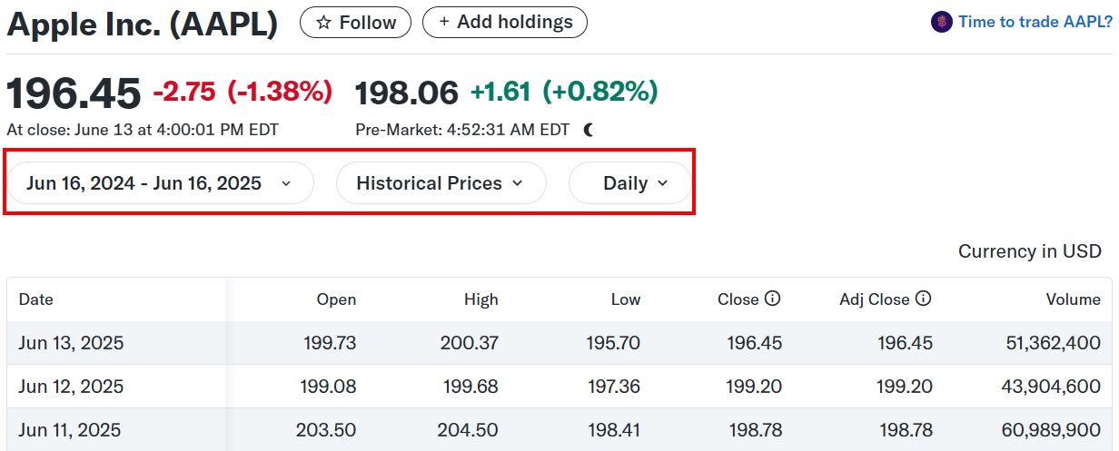
After the theory, let’s go through the practice. In this section, you’ll learn how to train a Deep Learning model to predict financial values. In particular, you’ll analyze the value of Apple in the stock market from Yahoo Finance.
Prerequisites and Dependencies
To reproduce this tutorial, your system has to match the following prerequisites:
Jupyter Notebook 6.x: You will use a Jupyter Notebook to analyze the data and make predictions with machine learning. Any version higher than 6.x will do.
Suppose you call your project’s folder predictive_analytics/. At the end of this step, it will have the following structure:
Perfect! Everything is set up for proceeding with the tutorial.
Before continuing with the article, I wanted to let you know that I've started my community in Circle. It’s a place where we can share our experiences and knowledge, and it’s included in your subscription. Enter the TWSC community at this link.
As you can see, the data is in a tabular format, and you have to retrieve the data from it. In particular, the CSS selector that defines the table is .table:
You can write the following code in the data_scraper.py file:
from selenium import webdriver
from selenium.webdriver.chrome.service import Service
from selenium.webdriver.support.ui import WebDriverWait
from selenium.webdriver.support import expected_conditions as EC
from selenium.webdriver.common.by import By
from selenium.common import NoSuchElementException
import pandas as pd
import os

# Configure Selenium
driver = webdriver.Chrome(service=Service())

# Target URL
url = "<https://finance.yahoo.com/quote/AAPL/history/?period1=1718528007&period2=1750063976>"
driver.get(url)

# Wait for the table to load
try:
    WebDriverWait(driver, 20).until(
        EC.presence_of_element_located((By.CSS_SELECTOR, ".table"))
    )
except NoSuchElementException:
    print("The table was not found, verify the HTML structure.")
    driver.quit()
    exit()

# Locate the table and extract its rows
table = driver.find_element(By.CSS_SELECTOR, ".table")
rows = table.find_elements(By.TAG_NAME, "tr")
This snippet sets up a Selenium Chrome driver instance, defines the target URL, and intercepts the whole table by using the dedicated CSS selector
Step #2: Retrieve the Data and Save it into a CSV File
You can now retrieve all the historical data selected and save it into a CSV file as follows:
# Extract headers from the first row of the table
headers = [header.text for header in rows[0].find_elements(By.TAG_NAME, "th")]

# Extract data from the subsequent rows
data = []
for row in rows[1:]:
    cols = [col.text for col in row.find_elements(By.TAG_NAME, "td")]
    if cols:
        data.append(cols)

# Convert data into a pandas DataFrame
df = pd.DataFrame(data, columns=headers)

# Determine the path to save the CSV file
current_dir = os.path.dirname(os.path.abspath(__file__))

# Navigate to the "data/" directory
data_dir = os.path.join(current_dir, "../data")

# Ensure the directory exists
os.makedirs(data_dir, exist_ok=True)

# Full path to the CSV file
csv_path = os.path.join(data_dir, "aapl_stock_data.csv")

# Save the DataFrame to the CSV file
df.to_csv(csv_path, index=False)
print(f"Historical stock data saved to {csv_path}")

# Close the WebDriver
driver.quit()
In this snippet:
The for loop extracts the data from all the rows in the table. The data is, then, saved as a Pandas dataframe with the method DataFrame().
The data is, then, saved as a CSV file in the directory data/ and the Chrome driver is closed.
Step #3: Launching the Script
From the main folder (predictive_analytics/), launch the scraper script with:
python scripts/data_scraper.py
At the end of the process, the dataset will be saved in data/aapl_stock_data.csv.
This is how the data in the CSV appears when you open it:
Very well! You retrieved and saved the historical data as a CSV. Now it’s time to go through the predictive analytics process.
The target value the model will predict is the “Adj Close”. In other words, given all the other values in input—the features—the model must be able to predict the adjusted close value. Note that there is no particular reason to choose this: you could choose the opening value (Open), the closing one (Close), or any other price value.
So, let’s see how to train a DL model that predicts its value, given all the others as input. But before doing so, let’s briefly describe how to use a Jupyter Notebook for the analysis.
Creating a New Jupyter Notebook Project
From the main folder (predictive_analytics/), navigate to the notebooks/ folder:
cd notebooks
From here, you can launch Jupyter Notebook:
jupyter notebook
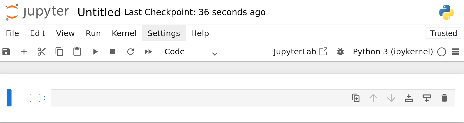
This command will open a new browser instance. Click on New > Python3 (ipykernel) to create a new Jupyter Notebook file:
This is what it looks like:
Click on Untitled and rename the file, for example, as analysis.ipynb:
Very well! You are now ready for the actual machine learning phase.
Step #1: Verify the Trend Over Time
As a first thing, let’s see the trend of the Adj Close value over time. To do so, write the following in a new cell of your Notebook and run it:
import pandas as pd
import matplotlib.pyplot as plt

# Path to the CSV file
csv_path = "../data/aapl_stock_data.csv"

# Open the CVS file
df = pd.read_csv(csv_path)

# Ensure the "Date" column is in datetime forma
df["Date"] = pd.to_datetime(df["Date"])

# Sort the data by date (if not already sorted)
df = df.sort_values(by="Date")

# Plot the "Adj Close" values over time
plt.figure(figsize=(10, 6))
plt.plot(df["Date"], df["Adj Close"], label="Adj Close", linewidth=2)

# Customize the plot
plt.title("AAPL Stock Adjusted Close Prices Over Time", fontsize=16) # Sets title
plt.xlabel("Date", fontsize=12) # Sets x-axis label
plt.ylabel("Adjusted Close Price (USD)", fontsize=12) # Sets y-axis label
plt.grid(True, linestyle="--", alpha=0.6) # Defines styles of the line
plt.legend(fontsize=12) # Shows legend
plt.tight_layout()

# Show the plot
plt.show()
The result is as follows:
Our goal is to find a model that can predict as best as it can this trend.
Step #2: Data Selection and Cleaning
Given the complete dataset you scraped and saved, you want to select all the features from it and be sure they are formatted correctly:
# Select all the features
features = ["Adj Close", "Open", "High", "Low", "Volume"]
df_features = df[features].copy()

# Convert Volume to a numeric type
df_features["Volume"] = pd.to_numeric(df_features["Volume"].astype(str).str.replace(",", ""), errors="coerce")

# Convert other columns just in case they are not numeric
for col in ["Adj Close", "Open", "High", "Low"]:
    df_features[col] = pd.to_numeric(df_features[col], errors='coerce')

# Handle any missing values that might have been created
df_features = df_features.interpolate()

# Scale all the selected features together
scaler = MinMaxScaler(feature_range=(0, 1))
scaled_data = scaler.fit_transform(df_features)
In this snippet, the key points are:
The pd.to_numeric() method that converts the values in every cell to numeric values.
The MinMaxScaler() method that scales all the numbers between 0 and 1. This is a best practice that allows you to work with numbers that are close to each other, for a simple reason: too big or too small numbers influence the training phase. However, it is normal to have numbers that are too small or too big because the features generally have different units of measure. In this case, for each row, the value of the volume is generally way bigger than the values of the other features (the prices).
Step #3: Data Splitting
Write the following in a new cell:
import numpy as np

# Create sequences of 60 time steps for prediction
sequence_length = 60
X, y = [], []

for i in range(sequence_length, len(scaled_data)):
    # X contains the last 60 days of all features
    X.append(scaled_data[i - sequence_length:i, :])
    # y is the 'Adj Close' price for the next day
    y.append(scaled_data[i, 0])

X, y = np.array(X), np.array(y)

# Split into training and test sets
split_index = int(len(X) * 0.8)  # 80% training, 20% testing
X_train, X_test = X[:split_index], X[split_index:]
y_train, y_test = y[:split_index], y[split_index:]
This cell is the heart of the process because the method int(len(X) * 0.8) splits the original dataset—the one you scraped—into two:
One is the training dataset, which is as big as 80% of the original one.
One is the test dataset—20% of the original.
So, in this step, you have created the famous training dataset.
Step #4: Train the Model
Now it’s time to train the model on the training dataset:
from tensorflow.keras.models import Sequential
from tensorflow.keras.layers import Dense, LSTM, Dropout
from tensorflow.keras.optimizers import Adam

# Build the model
model = Sequential()

# Layer 1: return sequences for the next LSTM layer
model.add(LSTM(units=100, return_sequences=True, activation='tanh', input_shape=(X_train.shape[1], X_train.shape[2])))
model.add(Dropout(0.2))

# Layer 2: return sequences for the next LSTM layer
model.add(LSTM(units=100, return_sequences=True, activation='tanh'))
model.add(Dropout(0.2))

# Layer 3: the final LSTM layer
model.add(LSTM(units=100, activation='tanh'))
model.add(Dropout(0.2))

# Dense Layer: A larger dense layer to interpret the LSTM outputs
model.add(Dense(units=50, activation='relu'))

# Output Layer: A single output neuron for the predicted price
model.add(Dense(units=1))

# Compile the model with a specific optimizer learning rate
optimizer = Adam(learning_rate=0.001)
model.compile(loss="mean_squared_error", optimizer=optimizer)

# Print a summary of the model
model.summary()

# Train the model
history = model.fit(
    X_train,
    y_train,
    epochs=100,  # Increased from 50 to 100
    batch_size=32,
    validation_data=(X_test, y_test),
    verbose=1
)
In this snippet:
You have used the Sequential() model. This needs different layers (I differentiated them with the comments).
The model is trained at the end of the cell using the fit() method. As you can see, inside it contains the parameters that represent the training dataset.
Now you are ready to see the first result!
Step #5: Calculate Numerical Results
Now, let’s see how good (or bad!) this model is at predicting the values
from sklearn.metrics import mean_squared_error, r2_score

# Make Predictions
y_pred_scaled = model.predict(X_test)

# Create array with the same number of columns as features
dummy_shape = (len(y_pred_scaled), scaled_data.shape[1])

# Un-scale the predictions
dummy_pred = np.zeros(shape=dummy_shape)
dummy_pred[:, 0] = y_pred_scaled.flatten()
y_pred = scaler.inverse_transform(dummy_pred)[:, 0]

# Un-scale the actual values
dummy_test = np.zeros(shape=dummy_shape)
dummy_test[:, 0] = y_test.flatten()
y_test_unscaled = scaler.inverse_transform(dummy_test)[:, 0]

# Evaluate the Model
mse = mean_squared_error(y_test_unscaled, y_pred)
r2 = r2_score(y_test_unscaled, y_pred)

# --- Print results ---
print("nLSTM Neural Network Results:")
print(f"Mean Squared Error: {mse:.2f}")
print(f"R-squared Score: {r2:.2f}")

# Reshape for plotting
y_test = y_test_unscaled.reshape(-1, 1)
y_pred = y_pred.reshape(-1, 1)
The important things in this cell are the following:
The model makes the predictions using the X_test array. In other words, it is calculating the values of the Adj Close column using the features in the test set.
The evaluation occurs via two metrics: the mean_squared_error() and the r2_score.
If the model is good, the expected values are near 0 for the mean squared error and near 1 for the R^2 score. Below is the result you can obtain:
Mean Squared Error: 33.63
R-squared Score: -0.12
So, you obtained a good value of the mean squared error, but not a good one or the R^2 score. However, the numerical validation is not always sufficient alone: we have, at least, to do a visual validation.
NOTE: Considering the statistical and stochastic nature of ML, you may obtain slightly different results.
Step #6: Visual Validation
For a visual validation, you want to see the trend over time of the actual values of the Adj Close column, taken on the test set, with respect to the predicted ones by the model. Below is how you can do so:
As you can see, the yellow-dotted lines (the values predicted by the model) do not fit the actual values (the blue line) very well. This means that the model used is not good enough to predict the Adj Close values, given the other values in the input.
What to do in such cases? Well, you generally have the following options:
Change the model.
Scrape more historical data.
Change the model and scrape more historical data.
The Web Scraping Club is a reader-supported publication. To receive new posts and support my work, consider becoming a free or paid subscriber.
A Discussion on the Process
So, what have you done so far in the previous tutorial? You have used a model that, given the input values, predicts the output (the value of the Adj Close). Let me clarify two concepts to help you get a broader overview:
In this tutorial, you just applied a DL model (with the method Sequential()). In the real world, this is not likely to be the common scenario. In reality, you will train different ML/DL models (generally, from 3 to 5 altogether) on the train set. Then, you will get the 2/3 that perform better on the train set, you will tune their hyperparameters—a passage we skipped here for simplicity—and see how they perform on the test set. From here, you will choose the one that performs best and deploy it into production.
After the deployment in production, you will need to test the performance of the model as new data comes in. If the model, at a certain point, performs bad you need to start the process from the beginning.
So, again, who’s the center of all of it? Well, of course, data and your capacity to set up an ETL (Extract Transform Load) pipeline that continuously scrapes the data that comes in, cleans it, and verifies the performance of the model.
So, as you can see…there is no magic in the process. Everything is just the integration of mathematics with software infrastructure and best practices!
Alternative Data: Expanding The Use Case on Web Scraping in Finance for Better Predictive Modeling
Since the tutorial is focused on the financial world, this is the perfect time to talk about a secret weapon where web scraping has a relevant usefulness. There's an entire industry on the web built around so-called “Alternative Data.”
So, what is it? Alternative data is information from non-traditional and non-financial sources, used to obtain a more complete and in-depth view of markets, companies, and consumers. In the context of financial stock prices prediction, it refers to any data that can provide insight into a company's performance that doesn't come from the company itself (like earnings reports, press releases, historical stock values, etc…). Think of it as gathering clues from the outside world to figure out what's happening on the inside. The goal is to predict key metrics—like future revenues, customer growth, or stock price movements—before that information becomes public knowledge.
We're talking about a huge range of information sources and, of course, web scraping plays a huge role here. It's the primary method for collecting many types of alternative data. In the context of stock price predictions, this data could be:
Hiring trends: Scraping a company's career page to see if they are aggressively hiring people (signaling expansion) or salespeople (signaling a push for revenue).
Product pricing and promotions: Tracking price changes on e-commerce sites to predict a company's profit margins or market position.
Website traffic and user engagement: Using data from different sources to estimate how many people are visiting a company's website, which can be a proxy for sales or user growth. But this could also involve scraping and analyzing engagement on social media company pages.
This is the ultimate application of predictive analytics on scraped data: turning public web data into a private, predictive insight to make better financial decisions. It perfectly illustrates how scraping unlocks data that is essential for building real-world financial predictive models. In fact, as you may know, the price itself is not the only metric investors use to predict future values—other than the market is unpredictable as we know; still, analysts and fund managers play an important role in this industry with their work.
Conclusion
In this article, you’ve learned what predictive analytics is, why web scraping is important to it, and how the process of scraping and predicting values works with a step-by-step tutorial.
So, out of curiosity…are you already using machine learning or deep learning algorithms on the data you scrape? Let’s discuss your experience in the comments!