The focus of this article is on anomaly detection on scraped data. We will first go through what “anomaly” means when referring to data, techniques you can use for intercepting anomalies, common anomalies in scraped data, and a practical implementation.
Let’s get started!
Before proceeding, let me thank Decodo, the platinum partner of the month, and their Scraping API.
Scraping made simple - try Decodo’s All-In-One Scraping API free for 7 days.
An anomaly is a data point, an event, or an observation that deviates significantly from the majority of the data you are analyzing. You can think of it as the "odd one out" in a dataset. These are often the most interesting and critical points of data because they can signify a unique event, an error, or a new, emerging trend.
You can intercept anomalies by their defining traits:
Rarity: Anomalies are infrequent by definition. If they occurred often, they would become part of the "normal" pattern. For example, in a dataset of credit card transactions, only an anomaly may mask a fraudulent payment.
Difference: They have features or values that are markedly different from the rest of the data. This difference can be in magnitude (a transaction for $10,000 when the average is $50) or in kind (a login from a new country).
Context-dependence: This is the most important point. What you can consider an anomaly is highly dependent on the context. For example, a spike in server traffic at 2:00 PM on a weekday might be normal. However, the exact same spike at 2:00 AM on a Sunday could be a significant anomaly.
So, the thing that you should read between the lines is that you get to know your data. When you know the data, the context, and the industry, you are the one who can define if a data point represents an anomaly, with respect to the common and expected behaviour.
Anomalies VS Outliers
Now, given the definitions above, you may ask yourself:” So, anomalies are just outliers, aren’t they?”. Well, yes and no. Let me drive you through the slight difference:
Outliers: An outlier is a data point that lies far from the rest of the data. They are often considered statistical noise and can be the result of data entry errors, measurement errors, or natural variations within the data distribution.
Anomalies: An anomaly is an outlier that carries potential meaning or signifies an unusual event, suspicious pattern, or critical issue. They are context-dependent and can result from real-world events like fraud, system failures, or unique occurrences.
So, mathematically speaking, they are the same: data points that significantly deviate from the mean value. This is why you get to know your data, context, and industry. When you find one (or more) data point that deviates from the “standard behaviour”, you have to evaluate if this is just an outlier or if it carries a real-world meaning.
For example, say you are analyzing purchases of a user who has a credit card they use to buy coffee for $5 every morning in San Francisco. Suddenly, a $2000 charge for electronics appears. Statistically, $2000 is an outlier if the mean purchase is $5 daily. So, you should investigate more to understand if that $2000 is an actual anomaly, due to a fraudulent purchase. In that case, if the store is on the opposite side of the world from San Francisco, that could be a strong indicator of fraud.
Types of Anomalies
Let’s remain in the mathematical field from now on. And let’s just use the term “anomaly” interchangeably with “outlier”. Anomalies can be categorized into the following:
Point anomalies (or global outliers): This is the most common and simplest type of anomaly. It is a single data point that is far outside the normal range of the entire dataset. For example, in a dataset of human body temperatures, a reading of 105°F (40.5°C) is a clear point anomaly. It is an extreme value regardless of any other factors.
Contextual anomalies (or conditional outliers): A data point that is considered anomalous only within a specific context. The value itself is not necessarily extreme, but it's unusual for the situation. For example, spending $200 on winter coats can be perfectly normal in October. However, spending the same $200 on winter coats in July in a hot climate could be a contextual anomaly—unless it was on sale (can you see how wide the context could be?).
Collective anomalies: It is a set of related data points that are not anomalous individually, but their occurrence together as a collection is anomalous. For instance, consider the heart rate from an EKG. A single beat might be within the normal range, but a long, sustained period where the heart rate is perfectly flat (a flatline) is a critical collective anomaly indicating cardiac arrest.
This episode is brought to you by our Gold Partners. Be sure to have a look at the Club Deals page to discover their generous offers available for the TWSC readers.
Until now, all straightforward. I defined what anomalies are and their relation to outliers. The question now is: how do you detect outliers in your data? Well, there are several options you can implement. Below is a very brief overview of the possibilities you have:
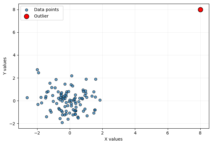
Visualization: Whenever possible, plotting your data is always a good idea. There are several graphs you can do—line plots, scatterplots, you name it. Anyhow, if outliers are present, they will be clearly visible regardless of the particular technique you used to plot your data. For example, the following is a scatterplot with one outlier (the red dot):
An outlier (red dot) in a scatterplot
Statistical methods: When data are numerical, you can spot outliers with mathematical methods. Or, you could identify outliers with a graphical method, and then use mathematical methods to quantify how much is the difference in value between the outlier and a reference value—the mean value of the dataset, for example. A common approach is the standard deviation method—also known as Z-Score method. You basically calculate the average and standard deviation of your data. Any data point that falls too many standard deviations away (more than 3 is a common choice) from the average is flagged as an anomaly.
Machine learning methods: Several machine learning methods are designed to intercept outliers in data. They are particularly suitable in cases where you can not apply statistical or graphical methods because the data is too complicated to analyze with them. Common solutions are:
Clustering techniques: These algorithms group similar data points into "clusters." Any data point that doesn't belong to a cluster or is very far from any cluster is considered an anomaly.
Isolation forest: This is a very efficient and popular method. It works by randomly "slicing" the dataset. The logic behind it is that anomalies are "few and different," so they are easier to isolate from the rest of the data points.
ARIMA/SARIMA models: ARIMA (and its counterpart, SARIMA) is the typical method for spotting outliers, particularly contextual anomalies, in time-series data. You train an ARIMA/SARIMA model on a historical dataset that you believe represents "normal" behavior. The model's entire purpose is to learn the underlying patterns in your data. You then use this trained model to make a forecast for the next time step(s). When the next actual data point arrives, you compare it to the forecast. If the actual value falls outside the prediction interval, it is flagged as an outlier.
As you can see, there are indeed several methodologies, each suitable for specific cases and circumstances.
Before continuing with the article, I wanted to let you know that I've started my community in Circle. It’s a place where we can share our experiences and knowledge, and it’s included in your subscription. Enter the TWSC community at this link.
Now, after all this discussion about data for data, let’s try to stick to web scraping. The point is that you can find outliers and anomalies in every dataset. So, the question now could be:” Are there any common scenarios where anomalies can be present in scraped data?”. The answer, of course, is yes. Let’s see common cases:
E-commerce and real estate: A common case you can face is the spikes in prices in e-commerce products or in real estate rent/selling prices. If you are scraping similar-priced products for comparing prices and find one (or a very few) that has a much higher or lower price than the mean, then you have your outlier. This is where you need to understand if the high difference in price is an actual outlier (a mistake in inserting the price in the platform) or a real anomaly (the price is really very far from the mean, for any reason. Maybe, the object is a second-hand).
Salaries in job positions: If you are searching for your next role and do not have a clear idea of what salary to expect or ask for during the negotiation, then scraping job offers and calculating the mean offered salary is a good solution. In this case, if you find an outlier, you can get a very interesting situation. You may have discovered a company with a recent quotation that really wants to invest in people, offering a much higher package. An application could be your life-changing occasion!
keyword in news/media/social media: If you scrape news or media websites, there can be days when a certain keyword is very recurrent. This can indicate a hot trend that makes sense to investigate more. The same thing applies to social media. If a keyword becomes common in comments on social media, then there can be the possibility of a trend around it.
Stock price or volume: This is something everyone probably thinks about when talking about anomalies in scraped data. Stock prices and volumes change every day, and an outlier can sometimes signify a change in the trend you do not want to miss if you are an investor (and use technical analysis to invest).
Missing content in scraped text: There are cases where you are analyzing the textual content you scraped, and part of it is simply missing. This is generally an anomaly because the cause is generally one of the two: something went wrong when scraping, or the content is actually missing in the source.
Implementing an Anomaly Detection Method on Scraped Data: Step-by-step Tutorial
Time to implement the theory into practice. The objective of the anomaly detection of this tutorial is NVIDIA’s stock price. But before going directly into the code, let’s first discuss what you should analyze and define.
Introductory Analysis
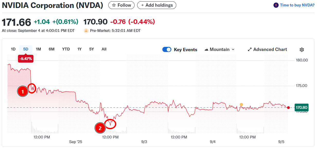
Whenever you scrape stock data, you first need to define the temporal interval. Let’s start by visualizing a 5-day chart:
Two potential anomalies in the NVDA stock price on the 5-day chart
By analyzing the above chart, you could say that there are two potential outliers (refer to the numbers in the red dots):
Number 1: This is where there is a high decrease in the price with a clear slope of the plot.
Number 2: After number 1, the price normalizes a bit. Then it goes down to number 2 and then normalizes again on a slightly higher value.
The point here is always the same as discussed before: What are you searching for? Are you searching for signals while live scraping? Are you training an ML model to intercept anomalies?
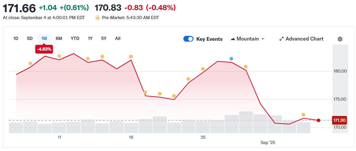
Also, what happens if you change the timeframe? Say you want to see a one-month price trend. Below is the plot:
The one-month price chart for the NVIDIA stock price
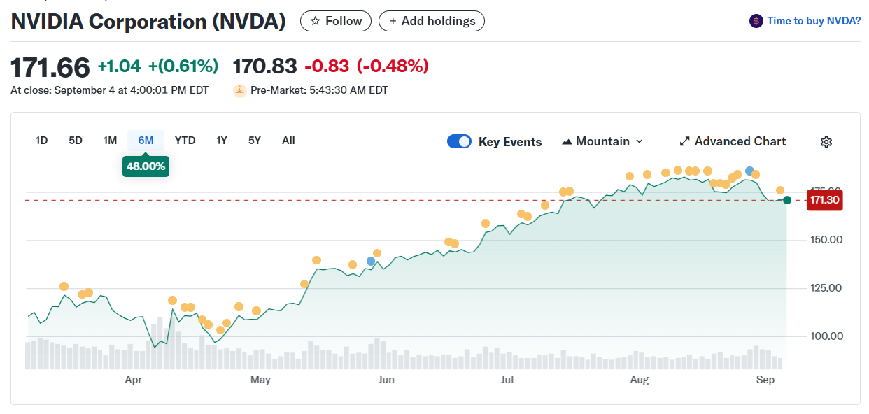
Considering the one-month plot, would you still consider points 1 and 2 as anomalies? And how about you change to a six-month one? Let’s see:
The six-month price chart for the NVIDIA stock price
Well, I think you get it…
So, let’s focus on the one-month plot and see what we can get using Isolation Forest.
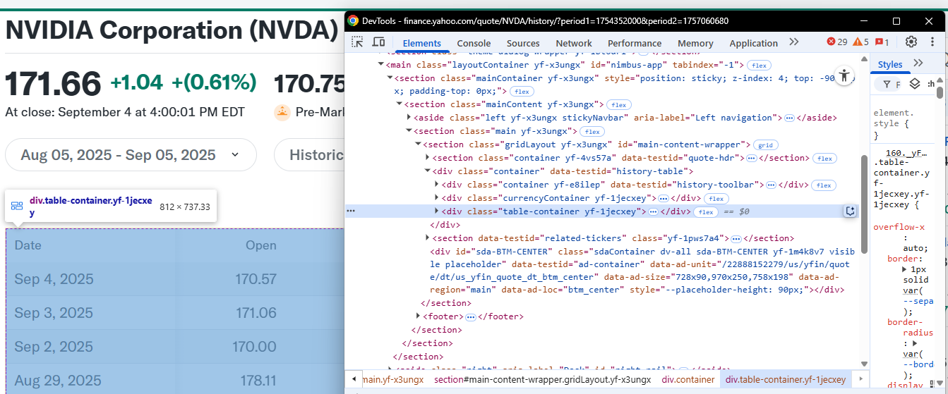
The data is in a tabular format, and you have to retrieve the data from it. In particular, the CSS selector that defines the table is .table:
The CSS selector of the table to scrape
Write the following code in the scraper.py file to extract the data and save it into a CSV file:
from selenium import webdriver
from selenium.webdriver.chrome.service import Service
from selenium.webdriver.support.ui import WebDriverWait
from selenium.webdriver.support import expected_conditions as EC
from selenium.webdriver.common.by import By
from selenium.common import NoSuchElementException
import os
import pandas as pd

# Configure Selenium
driver = webdriver.Chrome(service=Service())

# Target URL
url = "<https://finance.yahoo.com/quote/NVDA/history/?period1=1754352000&period2=1757060680>"
driver.get(url)

# Wait for the table to load
try:
    WebDriverWait(driver, 20).until(
        EC.presence_of_element_located((By.CSS_SELECTOR, ".table"))
    )
except NoSuchElementException:
    print("The table was not found, verify the HTML structure.")
    driver.quit()
    exit()

# Locate the table and extract its rows
table = driver.find_element(By.CSS_SELECTOR, ".table")
rows = table.find_elements(By.TAG_NAME, "tr")

# Extract headers from the first row of the table
headers = [header.text for header in rows[0].find_elements(By.TAG_NAME, "th")]

# Extract data from the subsequent rows
data = []
for row in rows[1:]:
    cols = [col.text for col in row.find_elements(By.TAG_NAME, "td")]
    if cols:
        data.append(cols)

# Convert data into a pandas DataFrame
df = pd.DataFrame(data, columns=headers)

# Determine the path to save the CSV file
current_dir = os.path.dirname(os.path.abspath(__file__))

# Navigate to the "data/" directory
data_dir = os.path.join(current_dir, "../data")

# Ensure the directory exists
os.makedirs(data_dir, exist_ok=True)

# Full path to the CSV file
csv_path = os.path.join(data_dir, "nvda_stock_data.csv")

# Save the DataFrame to the CSV file
df.to_csv(csv_path, index=False)
print(f"Historical stock data saved to {csv_path}")

# Close the WebDriver
driver.quit()
This code:
Launches a Selenium instance that scrapes the data from the target table.
Saves the data into a CSV file in the data/ folder.
When the script has completed its job, you will find a file named nvda_stock_data.csv in the data/ folder.
Very well! You scraped the target data successfully!
The Web Scraping Club is a reader-supported publication. To receive new posts and support my work, consider becoming a free or paid subscriber.
Step #2: Implement The Anomaly Detection With Isolation Forest
Data is scraped and saved into a CSV. To implement the anomaly detection, write the following code in the detector.py file:
import pandas as pd
from sklearn.ensemble import IsolationForest
import matplotlib.pyplot as plt

# Open CSV and verify target column is numeric
csv_path = "data/nvda_stock_data.csv"
df = pd.read_csv(csv_path)
df["Close"] = pd.to_numeric(df["Close"], errors="coerce")

# Prepare data for Isolation Forest
mask_valid = df["Close"].notna()
X = df.loc[mask_valid, ["Close"]].values

# Fit Isolation Forest
iso = IsolationForest(
    n_estimators=300,
    contamination=0.05,   # 5% anomalies; adjust as needed
    random_state=42,
    bootstrap=False
)
iso.fit(X)

# Get anomaly scores and predictions
scores = iso.decision_function(X)
preds = iso.predict(X)  # -1 = anomaly, 1 = normal

# Attach results to the original DataFrame
df.loc[mask_valid, "iso_score"] = scores
df.loc[mask_valid, "iso_pred"] = preds
df["is_anomaly"] = df["iso_pred"].eq(-1)

# Visualization
if "Date" in df.columns:
    # Try to parse dates for a nicer plot (optional)
    with pd.option_context("mode.chained_assignment", None):
        df["Date"] = pd.to_datetime(df["Date"], errors="coerce")

plt.figure(figsize=(12, 5))
plt.plot(df.index, df["Close"], label="Close", color="steelblue")
plt.scatter(
    df.index[df["is_anomaly"]],
    df.loc[df["is_anomaly"], "Close"],
    color="crimson",
    label="Anomaly",
    zorder=3
)
plt.title("Isolation Forest anomalies on Close")
plt.legend()
plt.tight_layout()
plt.show()
This code does the following:
Opens the CVS file that contains the scraped data.
Filters for the column “Close” and fits it to the Isolation Forest model. This means that you are searching for anomalies in the registered closing prices of NVIDIA stocks.
Calculates the anomaly and plots the trend over time of the closing price with the spotted anomalies.
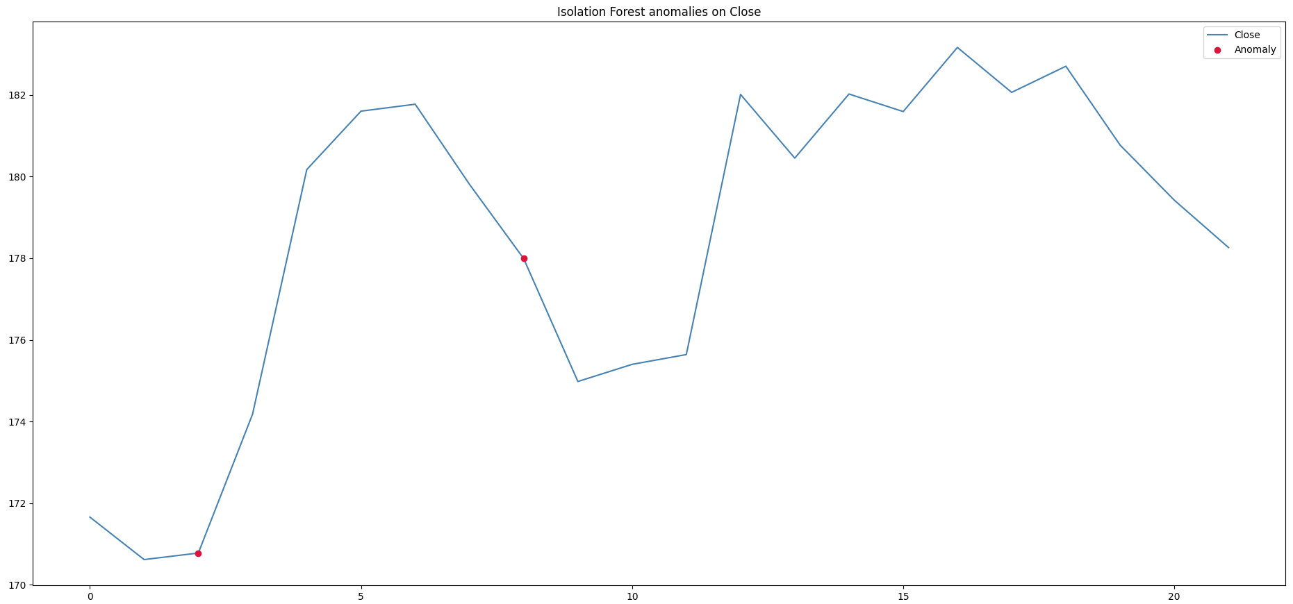
Below is the plot you will see when the program finishes its job:
Spotted anomalies in the NVIDIA stock closing price
So the model spotted two anomalies: one at the first date of the range, and one some days after. But why is that? What has the model done? Well, the key is in the contamination parameter that I set to 5%.
Isolation Forest assigns each point an “isolation score” by randomly splitting the data and measuring how quickly a point gets isolated in those random trees. In the above code, contamination=0.05 says: “treat about 5% of points as anomalies.” It is used only to set the decision threshold after the model computes scores.
Practically, with contamination=0.05 you are defining the fraction (≈5%) that will be flagged as anomalies on the training data.
So, first of all, if you change the value of the contamination parameter, you will obtain more (or less, depending if you increase or decrease it) anomaly points.
Secondly, remember that the code analyzes the “Close” column. So, you may ask yourself what happens if you consider another column. Let’s do so.
Step #3: Change Reference Column
Say you want to analyze the “Open” column. The code remains the same. You just need to substitute “Open” wherever you find “Close”. Below is the result, with the same contamination parameter:
Spotted anomalies in the NVIDIA stock opening price
There you go. The spotted anomalies are clearly two different datapoints from the previous ones! This remarks, once again, that anomalies are such depending on the context of what you are searching for.
Et voilà! You made it to intercept anomalies in scraped data.
Conclusion
In conclusion, in this article, I discussed the basic theory you need to understand anomaly detection. I also walked you through typical anomalies in scraped data and showed you how to implement an anomaly detection strategy after scraping data.
So, time to share! Have you ever had anomalies in your scraped data? Let us know in the comments!